Activity 19 Restoration of blurred image

Our final activity is again about image restoration. However unlike the previous activity, where we tackled images with additive noise, this time we will be restoring blurred images. Basically a blurred image is due to the effect of a degradation function to a given image. Let us also remember that in our earlier activities we have already encountered blurred images as a result of convolving apertures or filtering in the Fourier space. In this activity we will only be focused on blurred images caused by uniform linear motion with an additive gaussian noise.

Whatever the degradation process maybe, it can always be modeled as a convolution of the image and the degradation function such that in inverse space we obtained a blurred image given by

Equation 1

where H is the transfer function of the blurring process and N is the additive noise. For this activity we will be using the known degradation function of a uniform linear motion blur (equation 2). In equation 2, parameters a and b are the total displacements along x and y directions respectively and T is the total exposure time.

Equation 2

Just like in our previous activity the restoration process involves applying a filter or operation to obtain an estimate of the image from the degraded one. This time we will be using the Weiner (minimum mean square error) filter which incorporates both the degradation function and the statistics of the additive noise. The application of this filter operates in inverse space and is given by

Equation 3

where Sn and Sf are the power spectra of the noise and the ideal (undegraded) image. However, in real life situations it is highly improbable for us to have information on both the additive noise and the ideal (undegraded) image. For such cases equation 3 will be approximated into

Equation 4

where Sn/Sf is replaced by a constant K.

In this activity we use equations 1 and 2 on a gray scale image (figure 1) to produce a blurred image. Then we restore this blurred image using equation 3 or equation 4 with different values of K. We also do all of these for different gaussian noise strengths.

Figure 1

Figure 2. Blurred and restored image for different values of K, T, a, and b. We set the additive noise to be equal to zero

Figures 2 shows our results if we only have an image that is motioned blurred and no additive noise is present. From these images we clearly see that decreasing K improves the quality of our restoration. Furthermore, at the extreme case when K = 0 we arrive at a perfect restoration. These results are actually expected if we analyze equations 1 and 4. Doing simple math, at K = 0, equation 4 reduces to equation 5.

Equation 5

And since in this case we set the additive noise to zero, the last term in equation 5 vanishes and we are left with a perfect restoration.

(click to enlarge)
Figure 3. Blurred and restored image for different values of K, T, a, and b. Noise strength is sigma=0.001

In figure 3 we show the results of restoration when we consider the blurred image with an additive gaussian noise. Again similar to the case when there is no noise having a small value of K gives a very good quality of restoration. However, in this case if we further decrease K we then start to obtain dark noisy images. And, unlike the case of no noise, at K = 0 we obtain a meaningless restored image (almost pure noise).

One more notable result shown here is that even by using the exact power spectra of the noise and the original image, as in equation 3, we still do not obtain a perfect reconstruction. The restored image is indeed a significant improvement compared the blurred image but it is still not perfect.

I give myself a grade of 9 in this activity. The results we have obtained were very convincing but still left some questions unanswered. I would like to thank Master, Jaya, Orly, and Thirdy for helping me realize that I was wrong.


Main reference

A19 – Restoration of blurred image, AP186 2009

Activity 18 Noise models and basic image restoration

Just like any other measuring device or data gathering techniques noise is present in almost all forms of digital image acquisition. Noise, in general, is any unwanted aberration, random signal, or artifacts present in the image. Some of our previous activities already involved dealing with poor quality images using image enhancements. Previously we have used filtering in Fourier space, morphological operations, and even white balancing to improve the images. In this activity we will be using different image restoration methods to improve images with additive noise. In contrast to image enhancement, image restoration involves reversing the degradation process that produced the noise in the image. This means that a priori knowledge of the noise is important for a successful image restoration.

For this activity, we are tackling additive noise in the form of random variables following a specific probability distribution functions (PDF). We will be using six different noise models specifically: gaussian, rayleigh, gamma, exponential, uniform, and impulse noise.

Figure 1

There are many different types and methods of image restoration but in our case we will limit ourselves with spatial filters since they are most suited for additive noise. We will be using four types of filters namely, arithmetic, geometric, harmonic, and contraharmonic mean filters. With this filters we are basically changing the pixel values using the information provided by the image. All of this filters work by considering a subimage window centered at pixel(x,y) and using all the values within this window to calculate the new value of pixel(x,y) (figure 1). Equation 1 shows the formula followed by the arithmetic mean filter. This filter replaces the pixel value with the average of all the values in the window. On the other hand the geometric mean filter uses the product of all the values and takes its Ath root where A is the total area of the window (equation 2). The harmonic and contraharmonic mean filters follows equation 3 and 4 respectively.

Equation 1

Equation 2


Equation 3

Equation 4

In this activity we first create a noisy image by adding noise to a grayscale image then apply a restoration filter. We do this for each of the noise types and each of the restoration filters. Furthermore, to aide us in assessing our results we also take the histograms of all our images before and after restoration.

Figure 2 to 7 shows the result of applying the different restoration filters for each of the six noise types. It is clearly seen that even though the result is slightly more blurred it is actually much closer to the original image. This is further highlighted by looking at the image histograms. The histograms of the restored images are much closer that of the original image. The broadening or shifting introduced by the noise was greatly reduced by all the restoration filters. The minor blurring is simply due to the windowing; that is a smaller window results in less blurring but sacrifices the efficacy of the restoration. Here we used a 5x5 pixel window for a 256x256 pixel image.

Figure 2 Figure 3

Figure 4 Figure 5

Figure 6 Figure 7

However, looking at figure 7, we see that the restoration processes don't seem to negate the effect of the impulse (salt and pepper) noise. comparing the images we see very little to no improvement after implementing the arithmetic and geometric mean filters. Furthermore, looking at the histograms we even see that the restoration process degraded the image. The only semblance of improvement we can see is that the harmonic filtering and contraharmonic filtering with negative Q were both able to completely remove salt noise but not pepper. On the other hand using the contraharmonic filter with positive Q removes pepper noise but not salt.

We also did this whole procedure for a real grayscale image obtained from the internet (figure 8).

Figure 8

Overall this activity has been very enlightening and the results were very convincing. We were able to show that the different spatial filters are indeed useful for image restoration except for salt and pepper noise. I give myself a grade of 10 in this activity.

Main Reference:
AP186 "A18 – Noise models and basic image restoration", 2009

Activity 17 Photometric Stereo

Many of our previous activities involved using an objects reflectance, its interaction with a light source, to do color segmentation, white balancing, and even classification. In this activity we will again use the this phenomenon to reconstruct a 3D surface. The method we will be implementing is called photometric stereo.

To give us a better understanding of our method it is best to backtrack a little. Let us consider a camera, such as those we have benn using in our previous activities. Esentially, the image obtained by a camerais simply the light intensity, I, reflected by its subject which is dependent on the materials reflectance. However aside form its reflectance this intensity pattern is also dependent on the geometry of the object which results in light and dark (shadow) areas. This is much more understood by looking at figure 1, where we can see that the reflected intensity at point P is affected by the angle at which the light hits the surface, resulting to either a bright area and/or a shadow. Hence an intesity profile of an object also contains information on its geometry. Equation 1 gives an expression for this intensity where rho is the reflectance and k is a scaling parameter.

Figure 1. Visualization of Reflection on a 3D surface

Equation 1

Looking at our model on figure 1 and equation 1, it becomes apparent that we should also take into account the type or our light source. That is, point sources, line sources, and area sources would result in different reflected intensity patterns since the light coming from them would arrive at the surface differently (different angles and intensities as a function of distance). However in this activity we limit ourselves to an approximation that our point source is at infinity which results to equation 1 having the form

Equation 2.

Since we know the intensity profile from our image, if we have information on the location of the light source we can obtain the geometry of the surface by solving for the normal vector n.

In this method, photometric stereo, we will be using multiple images of the same object but with light sources at different locations to obtain an estimate of an objects 3 dimensional geometry. Since we have images for different light source locations we can rewrite equation 2 in matrix form where each row corresponds to a image (intensity profile) light source pair. Solving for the normal vector n we obtain

Equation 3

Equation 4

We also know that this normal vector n is related to the surface c by the taking the gradient of c such that

Equation 5

Finally we obtain the surface f(x,y) by integrating

Equation 6

We implement this algorithm in Scilab and make use of matrix properties and operation to reduce the computation time.

Figure 2. Images of the surface taken with 4 different location of the light source. Their respective locations were previously provided.

Figure 2 shows the raw images we used to calculate the 3D surface. We used 4 images with sources at different locations from the matlab file photos.mat. It is easily seen from this images that indeed there is a noticeable difference with different light source position.

Figure 3. 3D plot of the calculated surface of the 3D object. Errors are seen as spikes and dips over the surface

Using the algorithm we discussed and the raw images shown in figure 2 we reconstruct a hemispherical surface shown in figure 3. The resulting surface we obtained is in good agreement with our expectation. Notice that the shape is indeed that of a sphere and the background remains flat. However we also see that the surface is very rough and there is even a gentle dip in a the shape of a cross over the hemishpere. These imperfections is inherent to our method, since it is still only an approximation. A much better result may be obtained by having more images (hence more information resulting to a better approximation). Still overall we can say that the method is a success and is fairly simple to implement.

I give myself a grade of 10 in this activity. I thank Dr. Gay Pereze for her patience and useful adice.

Main Reference

A17– Photometric Stereo by Dr. Maricor Soriano, 2008

Activity 16 Neural Networks

Do you remember when I said machines are stupid? Well, I am not the first or the only one to believe so. Genius scientists and programmers that came before us also believed that machines and computers are sorely lacking when compared to the human brain. Just like in our pattern recognition activities (14 and 15), after creating our feature vectors we still needed to implement a formula so that the computer would classify the objects. So the brilliant scientists and programmers of the 19th century developed the “Neural Network”. The “Neural Network” works by mimicking how our own brain works; that is each neuron takes in multiple weighted inputs, processes the information, and then passes its output to a succeeding neuron. A collection of many interconnected neurons forms a “Neural Network.” The main advantage of using “Neural Network” over LDA and minimum distance classification is that we do not need to apply various classification rules and formulas.

Although I said that we do not use formulas with “Neural Network”, strictly speaking we still do. However this various calculations happen or exists within the structure of the network and the user won’t ever encounter it. We use “Neural Network” by simply giving it examples of a class and telling it that that particular example is a member of a specific class. For a given amount of time or iterations the “Neural Network” will adjusts the input weights of each neuron to minimize its error (identifying an object as a member of the wrong class). After all the iterations the “Neural Network” has already “learned” and will identify an object as a member of any class it has learned.

In this activity we will use Neural Networks from the ANN toolbox of SciLab to do pattern recognition. Our input to the neural network is the feature vectors we have from activities 14 and 15. We train the neural network by giving it 9 examples of each of the 4 classes and telling it which class each object belongs to (Activity 14 Table 1). Also we test the accuracy of the “Neural Network” network by letting it classify 40 more objects, one for each class, and counting how many it classified correctly. We test the accuracy of classification for different learning rates of the “Neural Network” from 0.01 to 0.99.

Table 1. Classification result and percent accuracy at different learning rates.
(click to enlarge)

Table 1 shows the results and accuracy of classification of the “Neural Network”. We see that as expected as we increase learning rate the accuracy of classification also increases and reaches a maximum of 100% at a learning rate of 0.23 to 0.55. The red box over table 1 highlights the area with 100% accuracy. However, as we increase the learning rate beyond 0.55 the accuracy slightly decrease to 97.5%. This is not expected since a higher learning rate should result in better classification. The classification accuracy versus learning rate is plotted in figure 1 and this trend of increase and slight decrease is observed much better.

Figure 1. Classification accuracy versus Neural Network learning rate. Red line highlights range with 100% accuracy

It would have been better to do multiple trials at different seed values to determine the standard deviation of the classification accuracy for each learning rate. If we have this information we might find out that this decrease in accuracy is not significant and is within the standard deviation. It would have also been better if we explored the effect of number of learning iterations but this was not explored due to time constraints.I would like to thank Kaye for reminding me of what to do in this activity. I give myself a grade of 10.

Main Reference:
Maricor Soriano, A16 – Neural Networks, AP186 2008
Cole’s AP186 Blog

Activity 15 Probabilistic Classification

In the previous activity we used minimum distance classification to assign the classes of our objects. However, even with our best choice of features, relying on the distances amongst feature vectors may still be ambiguous. This was not a problem in our previous activity but such a scenario is indeed possible. In activity 14 if we had just opted to use the normalized Red value and the Area/Perimeter^2 it would have been very difficult to differentiate between heart and diamond. In this activity we implement another method of classification called Linear Discriminant Analysis (LDA). We will still be using the same feature vectors that we described in activity 14 but this time we will use a different method for calculating an object’s class.

In pattern recognition we may think of the all the events as having a given probability. Let us consider two classes and a single object. Assuming that the object and the classes have similar features we may consider that the error or accuracy of our classification is given by the probability of assigning the object to the wrong or correct class. Moreover, the probability that an object came from a given class not only depends on its features but also the knowledge of how many objects belong to a given class. LDA is simply a method of calculating the probability of an object to belong to a given class using their features. The membership of an object is decided by the class that has the highest probability of containing it. The LDA method is based on the assumption that each class has a multivariate Normal distribution and that all the classes share the same Covariance matrix.

LDA calculates the probability, fij, of an object to belong in a class according to the equation

Equation 1

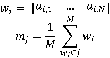
In this equation wi is the feature vector of object i and mj is the mean feature vector of class j. The value pj is the probability or ratio of the number of elements in class j over the total population of the classes.

Equation 2

Matrix C is the shared covariance matrix of all the classes and is calculated as the weighted mean of all the covariance matrices, cj, of the classes. We calculate the covariance matrix of each class following equation 3, where m is the mean feature vector of all the objects in all classes and Wj is the matrix containing all the feature vectors of all the members of class j. Finally nj is the number of membership in a given class.

Equation 3

Using the feature vectors we obtained in activity 14 we use LDA to classify the objects into the four classes of heart, diamond, spade, and club. We used the nine training objects in activity 14 to determine the covariance matrices and mean feature vector of the classes. All the raw data we used are shown in activity 14 Table 1 and Table 2.

Table 1. Resulting probability of each object per class and classification results.
(click to enlarge)

The result of our classification is shown on Table 1. Again we obtain a perfect 100% classification using this set of feature vectors. We however did not implement this method on the other 140 objects we used in activity 14. Still we believe that a very high classification accuracy will result if done so.

I give myself a grade of 10 in this activity. I want to thank Orly, Kaye, and Jaya for answering my questions.

Main Reference
Teknomo, Kardi. “Discriminant Analysis Tutorial”. http://people.revoledu.com/kardi/ tutorial/LDAKardi